Multiple Factor Parametric Tests - R
Contents
Multiple Factor Parametric Tests - R#
Factorial ANOVA#
Samples:
≥2Levels:
≥2Between or Within Subjects: Between
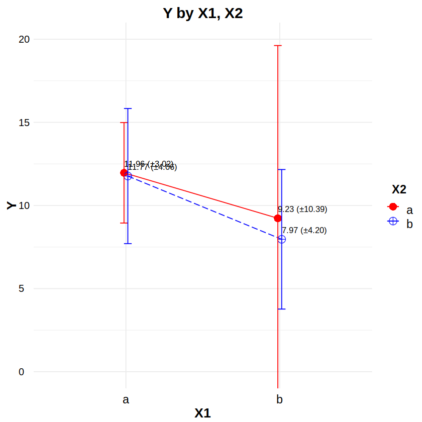
Reporting: “Figure 8 shows an interaction plot with ±1 standard deviation error bars for X1 and X2. A factorial ANOVA indicated a statistically significant effect on Y of X1 (F(1, 56) = 9.35, p < .01) and X2 (F(1, 56) = 4.30, p < .05), but not of the X1×X2 interaction (F(1, 56) = 0.42, n.s.).”
# Example data
# df has subjects (S), two between-Ss factors (X1,X2) each w/levels (a,b), and continuous response (Y)
df <- read.csv("data/2F2LBs.csv")
head(df, 20)
| S | X1 | X2 | Y | |
|---|---|---|---|---|
| <int> | <chr> | <chr> | <dbl> | |
| 1 | 1 | a | a | 9.939918 |
| 2 | 2 | a | b | 12.271865 |
| 3 | 3 | b | a | 11.062279 |
| 4 | 4 | b | b | 12.763591 |
| 5 | 5 | a | a | 7.980861 |
| 6 | 6 | a | b | 10.468626 |
| 7 | 7 | b | a | 21.071315 |
| 8 | 8 | b | b | 15.270048 |
| 9 | 9 | a | a | 22.125037 |
| 10 | 10 | a | b | 10.955709 |
| 11 | 11 | b | a | 14.496724 |
| 12 | 12 | b | b | 12.731080 |
| 13 | 13 | a | a | 14.110583 |
| 14 | 14 | a | b | 13.587539 |
| 15 | 15 | b | a | 13.175990 |
| 16 | 16 | b | b | 14.313530 |
| 17 | 17 | a | a | 11.595727 |
| 18 | 18 | a | b | 13.723466 |
| 19 | 19 | b | a | 17.276898 |
| 20 | 20 | b | b | 14.945042 |
library(ez) # for ezANOVA

df$S = factor(df$S) # Subject id is nominal
df$X1 = factor(df$X1) # X1 is a 2-level factor
df$X2 = factor(df$X2) # X2 is a 2-level factor

m = ezANOVA(dv=Y, between=c(X1,X2), wid=S, type=3, data=df) # use c() for >1 factors
m$Levene # if p<.05, we have a violation of homoscedasticity, so use a White-adjusted ANOVA
Coefficient covariances computed by hccm()
| DFn | DFd | SSn | SSd | F | p | p<.05 |
|---|---|---|---|---|---|---|
| <int> | <int> | <dbl> | <dbl> | <dbl> | <dbl> | <chr> |
| 3 | 56 | 36.93165 | 149.7687 | 4.603036 | 0.005989026 | * |
m= ezANOVA(dv=Y, between=c(X1,X2), wid=S, type=3, data=df, white.adjust=TRUE) # heteroscedastic
m$ANOVA
Coefficient covariances computed by hccm()
| Effect | DFn | DFd | F | p | p<.05 | |
|---|---|---|---|---|---|---|
| <chr> | <dbl> | <dbl> | <dbl> | <dbl> | <chr> | |
| 2 | X1 | 1 | 56 | 8.7309193 | 0.004569383 | * |
| 3 | X2 | 1 | 56 | 4.0094897 | 0.050096183 | |
| 4 | X1:X2 | 1 | 56 | 0.3876081 | 0.536086422 |
# the following also performs the same factorial ANOVA
m = aov(Y ~ X1*X2, data=df)
anova(m)
| Df | Sum Sq | Mean Sq | F value | Pr(>F) | |
|---|---|---|---|---|---|
| <int> | <dbl> | <dbl> | <dbl> | <dbl> | |
| X1 | 1 | 60.039468 | 60.039468 | 9.3545564 | 0.003408605 |
| X2 | 1 | 27.571854 | 27.571854 | 4.2958818 | 0.042819437 |
| X1:X2 | 1 | 2.665445 | 2.665445 | 0.4152944 | 0.521925508 |
| Residuals | 56 | 359.419527 | 6.418206 | NA | NA |
library(ggplot2)
library(ggthemes)
library(scales)
library(plyr)

# Interaction plot
# http://www.sthda.com/english/wiki/ggplot2-line-plot-quick-start-guide-r-software-and-data-visualization
# http://www.sthda.com/english/wiki/ggplot2-error-bars-quick-start-guide-r-software-and-data-visualization
# http://www.sthda.com/english/wiki/ggplot2-point-shapes
# http://www.sthda.com/english/wiki/ggplot2-line-types-how-to-change-line-types-of-a-graph-in-r-software
df2 <- ddply(df, ~ X1*X2, function(d) # make a summary data table
  c(NROW(d$Y),
    sum(is.na(d$Y)),
    sum(!is.na(d$Y)),
    mean(d$Y, na.rm=TRUE),
    sd(d$Y, na.rm=TRUE),
    median(d$Y, na.rm=TRUE),
    IQR(d$Y, na.rm=TRUE)))
colnames(df2) <- c("X1","X2","Rows","NAs","NotNAs","Mean","SD","Median","IQR")
ggplot(data=df2, aes(x=X1, y=Mean, color=X2, group=X2)) + theme_minimal() +
  # set the font styles for the plot title and axis titles
  theme(plot.title   = element_text(face="bold",  color="black", size=18, hjust=0.5, vjust=0.0, angle=0)) +
  theme(axis.title.x = element_text(face="bold",  color="black", size=16, hjust=0.5, vjust=0.0, angle=0)) +
  theme(axis.title.y = element_text(face="bold",  color="black", size=16, hjust=0.5, vjust=0.0, angle=90)) +
  # set the font styles for the value labels that show on each axis
  theme(axis.text.x  = element_text(face="plain", color="black", size=14, hjust=0.5, vjust=0.0, angle=0)) +
  theme(axis.text.y  = element_text(face="plain", color="black", size=12, hjust=0.0, vjust=0.5, angle=0)) +
  # set the font styles for the legend
  theme(legend.title = element_text(face="bold", color="black", size=14, hjust=0.5, vjust=0.0, angle=0)) +
  theme(legend.text  = element_text(face="plain", color="black", size=14, hjust=0.5, vjust=0.0, angle=0)) +
  # create the plot lines, points, and error bars
  geom_line(aes(linetype=X2), position=position_dodge(0.05)) +
  geom_point(aes(shape=X2, size=X2), position=position_dodge(0.05)) +
  geom_errorbar(aes(ymin=Mean-SD, ymax=Mean+SD), position=position_dodge(0.05), width=0.1) +
  # place text labels on each bar
  geom_text(aes(label=sprintf("%.2f (±%.2f)", Mean, SD)), position=position_dodge(0.05), hjust=0.0, vjust=-1.0, color="black", size=3.5) +
  # set the labels for the title and each axis
  labs(title="Y by X1, X2", x="X1", y="Y") +
  # set the ranges and value labels for each axis
  scale_x_discrete(labels=c("a","b")) +
  scale_y_continuous(breaks=seq(0,20,by=5), labels=seq(0,20,by=5), limits=c(0,20), oob=rescale_none) +
  # set the name, labels, and colors for the traces
  scale_color_manual(name="X2", labels=c("a","b"), values=c("red", "blue")) +
  # set the size and shape of the points
  scale_size_manual(values=c(4,4)) +
  scale_shape_manual(values=c(16,10)) +
  # set the linetype of the lines
  scale_linetype_manual(values=c("solid", "longdash"))

Linear Model (LM)#
Samples:
≥2Levels:
≥2Between or Within Subjects: Between
Reporting: “Figure 8 shows an interaction plot with ±1 standard deviation error bars for X1 and X2. An analysis of variance indicated a statistically significant effect on Y of X1 (F(1, 56) = 9.35, p < .01) and X2 (F(1, 56) = 4.30, p < .05), but not of the X1×X2 interaction (F(1, 56) = 0.42, n.s.).”
# Example data
# df has subjects (S), two between-Ss factors (X1,X2) each w/levels (a,b), and continuous response (Y)
df <- read.csv("data/2F2LBs.csv")
head(df, 20)
| S | X1 | X2 | Y | |
|---|---|---|---|---|
| <int> | <chr> | <chr> | <dbl> | |
| 1 | 1 | a | a | 9.939918 |
| 2 | 2 | a | b | 12.271865 |
| 3 | 3 | b | a | 11.062279 |
| 4 | 4 | b | b | 12.763591 |
| 5 | 5 | a | a | 7.980861 |
| 6 | 6 | a | b | 10.468626 |
| 7 | 7 | b | a | 21.071315 |
| 8 | 8 | b | b | 15.270048 |
| 9 | 9 | a | a | 22.125037 |
| 10 | 10 | a | b | 10.955709 |
| 11 | 11 | b | a | 14.496724 |
| 12 | 12 | b | b | 12.731080 |
| 13 | 13 | a | a | 14.110583 |
| 14 | 14 | a | b | 13.587539 |
| 15 | 15 | b | a | 13.175990 |
| 16 | 16 | b | b | 14.313530 |
| 17 | 17 | a | a | 11.595727 |
| 18 | 18 | a | b | 13.723466 |
| 19 | 19 | b | a | 17.276898 |
| 20 | 20 | b | b | 14.945042 |
df$S = factor(df$S) # Subject id is nominal (unused)
df$X1 = factor(df$X1) # X1 is a 2-level factor
df$X2 = factor(df$X2) # X2 is a 2-level factor
m = lm(Y ~ X1*X2, data=df)
anova(m)
| Df | Sum Sq | Mean Sq | F value | Pr(>F) | |
|---|---|---|---|---|---|
| <int> | <dbl> | <dbl> | <dbl> | <dbl> | |
| X1 | 1 | 60.039468 | 60.039468 | 9.3545564 | 0.003408605 |
| X2 | 1 | 27.571854 | 27.571854 | 4.2958818 | 0.042819437 |
| X1:X2 | 1 | 2.665445 | 2.665445 | 0.4152944 | 0.521925508 |
| Residuals | 56 | 359.419527 | 6.418206 | NA | NA |
library(ggplot2)
library(ggthemes)
library(scales)
library(plyr)

# Interaction plot
# http://www.sthda.com/english/wiki/ggplot2-line-plot-quick-start-guide-r-software-and-data-visualization
# http://www.sthda.com/english/wiki/ggplot2-error-bars-quick-start-guide-r-software-and-data-visualization
# http://www.sthda.com/english/wiki/ggplot2-point-shapes
# http://www.sthda.com/english/wiki/ggplot2-line-types-how-to-change-line-types-of-a-graph-in-r-software
df2 <- ddply(df, ~ X1*X2, function(d) # make a summary data table
  c(NROW(d$Y),
    sum(is.na(d$Y)),
    sum(!is.na(d$Y)),
    mean(d$Y, na.rm=TRUE),
    sd(d$Y, na.rm=TRUE),
    median(d$Y, na.rm=TRUE),
    IQR(d$Y, na.rm=TRUE)))
colnames(df2) <- c("X1","X2","Rows","NAs","NotNAs","Mean","SD","Median","IQR")
ggplot(data=df2, aes(x=X1, y=Mean, color=X2, group=X2)) + theme_minimal() +
  # set the font styles for the plot title and axis titles
  theme(plot.title   = element_text(face="bold",  color="black", size=18, hjust=0.5, vjust=0.0, angle=0)) +
  theme(axis.title.x = element_text(face="bold",  color="black", size=16, hjust=0.5, vjust=0.0, angle=0)) +
  theme(axis.title.y = element_text(face="bold",  color="black", size=16, hjust=0.5, vjust=0.0, angle=90)) +
  # set the font styles for the value labels that show on each axis
  theme(axis.text.x  = element_text(face="plain", color="black", size=14, hjust=0.5, vjust=0.0, angle=0)) +
  theme(axis.text.y  = element_text(face="plain", color="black", size=12, hjust=0.0, vjust=0.5, angle=0)) +
  # set the font styles for the legend
  theme(legend.title = element_text(face="bold", color="black", size=14, hjust=0.5, vjust=0.0, angle=0)) +
  theme(legend.text  = element_text(face="plain", color="black", size=14, hjust=0.5, vjust=0.0, angle=0)) +
  # create the plot lines, points, and error bars
  geom_line(aes(linetype=X2), position=position_dodge(0.05)) +
  geom_point(aes(shape=X2, size=X2), position=position_dodge(0.05)) +
  geom_errorbar(aes(ymin=Mean-SD, ymax=Mean+SD), position=position_dodge(0.05), width=0.1) +
  # place text labels on each bar
  geom_text(aes(label=sprintf("%.2f (±%.2f)", Mean, SD)), position=position_dodge(0.05), hjust=0.0, vjust=-1.0, color="black", size=3.5) +
  # set the labels for the title and each axis
  labs(title="Y by X1, X2", x="X1", y="Y") +
  # set the ranges and value labels for each axis
  scale_x_discrete(labels=c("a","b")) +
  scale_y_continuous(breaks=seq(0,20,by=5), labels=seq(0,20,by=5), limits=c(0,20), oob=rescale_none) +
  # set the name, labels, and colors for the traces
  scale_color_manual(name="X2", labels=c("a","b"), values=c("red", "blue")) +
  # set the size and shape of the points
  scale_size_manual(values=c(4,4)) +
  scale_shape_manual(values=c(16,10)) +
  # set the linetype of the lines
  scale_linetype_manual(values=c("solid", "longdash"))
Factorial Repeated Measures ANOVA#
Samples:
≥2Levels:
≥2Between or Within Subjects: Within
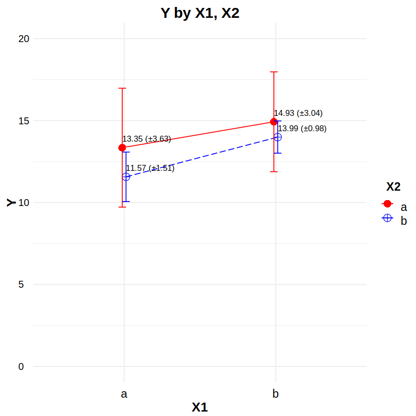
Reporting: “Figure 9 shows an interaction plot with ±1 standard deviation error bars for X1 and X2. A factorial repeated measures ANOVA indicated a statistically significant effect on Y of X1 (F(1, 14) = 5.45, p < .05), but not of X2 (F(1, 14) = 0.18, n.s.), or of the X1×X2 interaction (F(1, 14) = 0.12, n.s.).”
# Example data
# df has subjects (S), two within-Ss factors (X1,X2) each w/levels (a,b), and continuous response (Y)
df <- read.csv("data/2F2LWs.csv")
head(df, 20)
| S | X1 | X2 | Y | |
|---|---|---|---|---|
| <int> | <chr> | <chr> | <dbl> | |
| 1 | 1 | a | a | 11.4749213 |
| 2 | 1 | a | b | 14.8431021 |
| 3 | 1 | b | a | 0.1430649 |
| 4 | 1 | b | b | 15.0210806 |
| 5 | 2 | a | a | 16.9487115 |
| 6 | 2 | a | b | 12.9088880 |
| 7 | 2 | b | a | 7.3433619 |
| 8 | 2 | b | b | 11.1885220 |
| 9 | 3 | a | a | 12.3397073 |
| 10 | 3 | a | b | 14.8390688 |
| 11 | 3 | b | a | 21.5131754 |
| 12 | 3 | b | b | 0.2390247 |
| 13 | 4 | a | a | 11.7081257 |
| 14 | 4 | a | b | 13.8740498 |
| 15 | 4 | b | a | 4.3615137 |
| 16 | 4 | b | b | 2.3686943 |
| 17 | 5 | a | a | 15.3668561 |
| 18 | 5 | a | b | 13.6340391 |
| 19 | 5 | b | a | 4.9401806 |
| 20 | 5 | b | b | 13.5781464 |
library(ez) # for ezANOVA

df$S = factor(df$S) # Subject id is nominal
df$X1 = factor(df$X1) # X1 is a 2-level factor
df$X2 = factor(df$X2) # X2 is a 2-level factor

m = ezANOVA(dv=Y, within=c(X1,X2), wid=S, type=3, data=df) # use c() for >1 factors
m$Mauchly # p<.05 indicates a sphericity violation
NULL
m$ANOVA # use if no violation
| Effect | DFn | DFd | F | p | p<.05 | ges | |
|---|---|---|---|---|---|---|---|
| <chr> | <dbl> | <dbl> | <dbl> | <dbl> | <chr> | <dbl> | |
| 2 | X1 | 1 | 14 | 5.4537088 | 0.03492658 | * | 0.070392015 |
| 3 | X2 | 1 | 14 | 0.1797949 | 0.67799256 | 0.003762924 | |
| 4 | X1:X2 | 1 | 14 | 0.1223175 | 0.73173975 | 0.002019078 |
# if there is a sphericity violation, report the Greenhouse-Geisser or Huynh-Feldt correction
p = match(m$Sphericity$Effect, m$ANOVA$Effect) # positions of within-Ss effects in m$ANOVA
m$Sphericity$GGe.DFn = m$Sphericity$GGe * m$ANOVA$DFn[p] # Greenhouse-Geisser DFs
m$Sphericity$GGe.DFd = m$Sphericity$GGe * m$ANOVA$DFd[p]
m$Sphericity$HFe.DFn = m$Sphericity$HFe * m$ANOVA$DFn[p] # Huynh-Feldt DFs
m$Sphericity$HFe.DFd = m$Sphericity$HFe * m$ANOVA$DFd[p]
m$Sphericity # show results
- $GGe.DFn
- $GGe.DFd
- $HFe.DFn
- $HFe.DFd
# the following also performs the equivalent repeated measures ANOVA, but does not address sphericity
m = aov(Y ~ X1*X2 + Error(S/(X1*X2)), data=df)
summary(m)
Error: S
          Df Sum Sq Mean Sq F value Pr(>F)
Residuals 14  592.5   42.32

Error: S:X1
          Df Sum Sq Mean Sq F value Pr(>F)
X1         1  160.3  160.28   5.454 0.0349 *
Residuals 14  411.4   29.39
---
Signif. codes:  0 ‘***’ 0.001 ‘**’ 0.01 ‘*’ 0.05 ‘.’ 0.1 ‘ ’ 1

Error: S:X2
          Df Sum Sq Mean Sq F value Pr(>F)
X2         1    8.0    8.00    0.18  0.678
Residuals 14  622.5   44.47

Error: S:X1:X2
          Df Sum Sq Mean Sq F value Pr(>F)
X1:X2      1    4.3    4.28   0.122  0.732
Residuals 14  490.1   35.01
# Interaction plot
# http://www.sthda.com/english/wiki/ggplot2-line-plot-quick-start-guide-r-software-and-data-visualization
# http://www.sthda.com/english/wiki/ggplot2-error-bars-quick-start-guide-r-software-and-data-visualization
# http://www.sthda.com/english/wiki/ggplot2-point-shapes
# http://www.sthda.com/english/wiki/ggplot2-line-types-how-to-change-line-types-of-a-graph-in-r-software
df2 <- ddply(df, ~ X1*X2, function(d) # make a summary data table
  c(NROW(d$Y),
    sum(is.na(d$Y)),
    sum(!is.na(d$Y)),
    mean(d$Y, na.rm=TRUE),
    sd(d$Y, na.rm=TRUE),
    median(d$Y, na.rm=TRUE),
    IQR(d$Y, na.rm=TRUE)))
colnames(df2) <- c("X1","X2","Rows","NAs","NotNAs","Mean","SD","Median","IQR")
ggplot(data=df2, aes(x=X1, y=Mean, color=X2, group=X2)) + theme_minimal() +
  # set the font styles for the plot title and axis titles
  theme(plot.title   = element_text(face="bold",  color="black", size=18, hjust=0.5, vjust=0.0, angle=0)) +
  theme(axis.title.x = element_text(face="bold",  color="black", size=16, hjust=0.5, vjust=0.0, angle=0)) +
  theme(axis.title.y = element_text(face="bold",  color="black", size=16, hjust=0.5, vjust=0.0, angle=90)) +
  # set the font styles for the value labels that show on each axis
  theme(axis.text.x  = element_text(face="plain", color="black", size=14, hjust=0.5, vjust=0.0, angle=0)) +
  theme(axis.text.y  = element_text(face="plain", color="black", size=12, hjust=0.0, vjust=0.5, angle=0)) +
  # set the font styles for the legend
  theme(legend.title = element_text(face="bold", color="black", size=14, hjust=0.5, vjust=0.0, angle=0)) +
  theme(legend.text  = element_text(face="plain", color="black", size=14, hjust=0.5, vjust=0.0, angle=0)) +
  # create the plot lines, points, and error bars
  geom_line(aes(linetype=X2), position=position_dodge(0.05)) +
  geom_point(aes(shape=X2, size=X2), position=position_dodge(0.05)) +
  geom_errorbar(aes(ymin=Mean-SD, ymax=Mean+SD), position=position_dodge(0.05), width=0.1) +
  # place text labels on each bar
  geom_text(aes(label=sprintf("%.2f (±%.2f)", Mean, SD)), position=position_dodge(0.05), hjust=0.0, vjust=-1.0, color="black", size=3.5) +
  # set the labels for the title and each axis
  labs(title="Y by X1, X2", x="X1", y="Y") +
  # set the ranges and value labels for each axis
  scale_x_discrete(labels=c("a","b")) +
  scale_y_continuous(breaks=seq(0,20,by=5), labels=seq(0,20,by=5), limits=c(0,20), oob=rescale_none) +
  # set the name, labels, and colors for the traces
  scale_color_manual(name="X2", labels=c("a","b"), values=c("red", "blue")) +
  # set the size and shape of the points
  scale_size_manual(values=c(4,4)) +
  scale_shape_manual(values=c(16,10)) +
  # set the linetype of the lines
  scale_linetype_manual(values=c("solid", "longdash"))

Linear Mixed Model (LMM)#
Samples:
≥2Levels:
≥2Between or Within Subjects: Within
Reporting: “Figure 9 shows an interaction plot with ±1 standard deviation error bars for X1 and X2. A linear mixed model analysis of variance indicated a statistically significant effect on Y of X1 (F(1, 42) = 4.42, p < .05), but not of X2 (F(1, 42) = 0.22, n.s.), or of the X1×X2 interaction (F(1, 42) = 0.12, n.s.).”
# Example data
# df has subjects (S), two within-Ss factors (X1,X2) each w/levels (a,b), and continuous response (Y)
df <- read.csv("data/2F2LWs.csv")
head(df, 20)
| S | X1 | X2 | Y | |
|---|---|---|---|---|
| <int> | <chr> | <chr> | <dbl> | |
| 1 | 1 | a | a | 11.4749213 |
| 2 | 1 | a | b | 14.8431021 |
| 3 | 1 | b | a | 0.1430649 |
| 4 | 1 | b | b | 15.0210806 |
| 5 | 2 | a | a | 16.9487115 |
| 6 | 2 | a | b | 12.9088880 |
| 7 | 2 | b | a | 7.3433619 |
| 8 | 2 | b | b | 11.1885220 |
| 9 | 3 | a | a | 12.3397073 |
| 10 | 3 | a | b | 14.8390688 |
| 11 | 3 | b | a | 21.5131754 |
| 12 | 3 | b | b | 0.2390247 |
| 13 | 4 | a | a | 11.7081257 |
| 14 | 4 | a | b | 13.8740498 |
| 15 | 4 | b | a | 4.3615137 |
| 16 | 4 | b | b | 2.3686943 |
| 17 | 5 | a | a | 15.3668561 |
| 18 | 5 | a | b | 13.6340391 |
| 19 | 5 | b | a | 4.9401806 |
| 20 | 5 | b | b | 13.5781464 |
library(lme4) # for lmer
library(car) # for Anova
df$S = factor(df$S) # Subject id is nominal
df$X1 = factor(df$X1) # X1 is a 2-level factor
df$X2 = factor(df$X2) # X2 is a 2-level factor
contrasts(df$X1) <- "contr.sum"
contrasts(df$X2) <- "contr.sum"
m = lmer(Y ~ X1*X2 + (1|S), data=df)
Anova(m, type=3, test.statistic="F")
Loading required package: Matrix
Loading required package: carData
| F | Df | Df.res | Pr(>F) | |
|---|---|---|---|---|
| <dbl> | <dbl> | <dbl> | <dbl> | |
| (Intercept) | 148.4297541 | 1 | 14 | 7.698544e-09 |
| X1 | 4.4167657 | 1 | 42 | 4.162596e-02 |
| X2 | 0.2203147 | 1 | 42 | 6.412279e-01 |
| X1:X2 | 0.1180081 | 1 | 42 | 7.329188e-01 |
# Interaction plot
# http://www.sthda.com/english/wiki/ggplot2-line-plot-quick-start-guide-r-software-and-data-visualization
# http://www.sthda.com/english/wiki/ggplot2-error-bars-quick-start-guide-r-software-and-data-visualization
# http://www.sthda.com/english/wiki/ggplot2-point-shapes
# http://www.sthda.com/english/wiki/ggplot2-line-types-how-to-change-line-types-of-a-graph-in-r-software
df2 <- ddply(df, ~ X1*X2, function(d) # make a summary data table
  c(NROW(d$Y),
    sum(is.na(d$Y)),
    sum(!is.na(d$Y)),
    mean(d$Y, na.rm=TRUE),
    sd(d$Y, na.rm=TRUE),
    median(d$Y, na.rm=TRUE),
    IQR(d$Y, na.rm=TRUE)))
colnames(df2) <- c("X1","X2","Rows","NAs","NotNAs","Mean","SD","Median","IQR")
ggplot(data=df2, aes(x=X1, y=Mean, color=X2, group=X2)) + theme_minimal() +
  # set the font styles for the plot title and axis titles
  theme(plot.title   = element_text(face="bold",  color="black", size=18, hjust=0.5, vjust=0.0, angle=0)) +
  theme(axis.title.x = element_text(face="bold",  color="black", size=16, hjust=0.5, vjust=0.0, angle=0)) +
  theme(axis.title.y = element_text(face="bold",  color="black", size=16, hjust=0.5, vjust=0.0, angle=90)) +
  # set the font styles for the value labels that show on each axis
  theme(axis.text.x  = element_text(face="plain", color="black", size=14, hjust=0.5, vjust=0.0, angle=0)) +
  theme(axis.text.y  = element_text(face="plain", color="black", size=12, hjust=0.0, vjust=0.5, angle=0)) +
  # set the font styles for the legend
  theme(legend.title = element_text(face="bold", color="black", size=14, hjust=0.5, vjust=0.0, angle=0)) +
  theme(legend.text  = element_text(face="plain", color="black", size=14, hjust=0.5, vjust=0.0, angle=0)) +
  # create the plot lines, points, and error bars
  geom_line(aes(linetype=X2), position=position_dodge(0.05)) +
  geom_point(aes(shape=X2, size=X2), position=position_dodge(0.05)) +
  geom_errorbar(aes(ymin=Mean-SD, ymax=Mean+SD), position=position_dodge(0.05), width=0.1) +
  # place text labels on each bar
  geom_text(aes(label=sprintf("%.2f (±%.2f)", Mean, SD)), position=position_dodge(0.05), hjust=0.0, vjust=-1.0, color="black", size=3.5) +
  # set the labels for the title and each axis
  labs(title="Y by X1, X2", x="X1", y="Y") +
  # set the ranges and value labels for each axis
  scale_x_discrete(labels=c("a","b")) +
  scale_y_continuous(breaks=seq(0,20,by=5), labels=seq(0,20,by=5), limits=c(0,20), oob=rescale_none) +
  # set the name, labels, and colors for the traces
  scale_color_manual(name="X2", labels=c("a","b"), values=c("red", "blue")) +
  # set the size and shape of the points
  scale_size_manual(values=c(4,4)) +
  scale_shape_manual(values=c(16,10)) +
  # set the linetype of the lines
  scale_linetype_manual(values=c("solid", "longdash"))