ANOVA Assumptions - R#

Shapiro-Wilk Test (on responses)#

Assumption: Normality
Context of Use: t-test, ANOVA, LM, LMM
Reporting: “To test the assumption of conditional normality, a Shapiro-Wilk test was run on the response Y for each combination of levels of factors X1 and X2. All combinations were found to be statistically non-significant except condition (b,b), which showed a statistically significant deviation from normality (W = .794, p < .01).”

# Example data
# df has two factors (X1,X2) each w/two levels (a,b) and continuous response Y
df <- read.csv("data/2F2LBs_normal.csv")
head(df, 20)

A data.frame: 20 × 4
	S	X1	X2	Y
	<int>	<chr>	<chr>	<dbl>
1	1	a	a	11.867340
2	2	a	b	15.453745
3	3	b	a	15.782415
4	4	b	b	13.626554
5	5	a	a	11.608195
6	6	a	b	19.540674
7	7	b	a	15.878829
8	8	b	b	16.654611
9	9	a	a	17.370245
10	10	a	b	17.547025
11	11	b	a	19.423109
12	12	b	b	16.369147
13	13	a	a	22.896627
14	14	a	b	14.037504
15	15	b	a	15.564130
16	16	b	b	16.109281
17	17	a	a	7.028036
18	18	a	b	21.508059
19	19	b	a	17.644257
20	20	b	b	16.054999

## Shapiro-Wilk conditional normality test
# (on the response within each condition)
shapiro.test(df[df$X1 == "a" & df$X2 == "a",]$Y) # condition a,a
shapiro.test(df[df$X1 == "a" & df$X2 == "b",]$Y) # condition a,b
shapiro.test(df[df$X1 == "b" & df$X2 == "a",]$Y) # condition b,a
shapiro.test(df[df$X1 == "b" & df$X2 == "b",]$Y) # condition b,b

	Shapiro-Wilk normality test

data:  df[df$X1 == "a" & df$X2 == "a", ]$Y
W = 0.97554, p-value = 0.93

	Shapiro-Wilk normality test

data:  df[df$X1 == "a" & df$X2 == "b", ]$Y
W = 0.93417, p-value = 0.3147

	Shapiro-Wilk normality test

data:  df[df$X1 == "b" & df$X2 == "a", ]$Y
W = 0.98454, p-value = 0.9914

	Shapiro-Wilk normality test

data:  df[df$X1 == "b" & df$X2 == "b", ]$Y
W = 0.7938, p-value = 0.003064

Shapiro-Wilk Test (on residuals)#

Assumption: Normality
Context of Use: t-test, ANOVA, LM, LMM
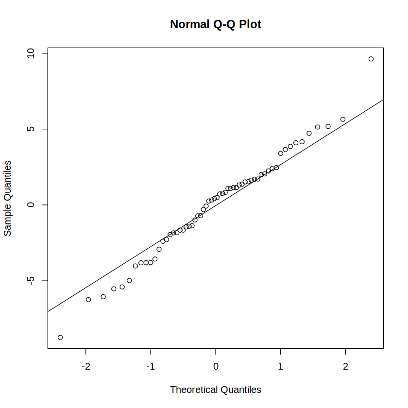
Reporting: “To test the normality assumption, a Shapiro-Wilk test was run on the residuals of a between-subjects full-factorial ANOVA model. The test was statistically non-significant (W = .988, p = .798), indicating compliance with the normality assumption. A Q-Q plot of residuals visually confirms the same (Figure 1).”

# Example data
# df has two factors (X1,X2) each w/two levels (a,b) and continuous response Y
df <- read.csv("data/2F2LBs_normal.csv")
head(df, 20)

A data.frame: 20 × 4
	S	X1	X2	Y
	<int>	<chr>	<chr>	<dbl>
1	1	a	a	11.867340
2	2	a	b	15.453745
3	3	b	a	15.782415
4	4	b	b	13.626554
5	5	a	a	11.608195
6	6	a	b	19.540674
7	7	b	a	15.878829
8	8	b	b	16.654611
9	9	a	a	17.370245
10	10	a	b	17.547025
11	11	b	a	19.423109
12	12	b	b	16.369147
13	13	a	a	22.896627
14	14	a	b	14.037504
15	15	b	a	15.564130
16	16	b	b	16.109281
17	17	a	a	7.028036
18	18	a	b	21.508059
19	19	b	a	17.644257
20	20	b	b	16.054999

m = aov(Y ~ X1*X2, data=df) # make anova model
shapiro.test(residuals(m))

	Shapiro-Wilk normality test

data:  residuals(m)
W = 0.98751, p-value = 0.7979

par(mfrow=c(1,1))
qqnorm(residuals(m)); qqline(residuals(m)) # Q-Q plot

Anderson-Darling Test (on responses)#

Assumption: Normality
Context of Use: t-test, ANOVA, LM, LMM
Reporting: “To test the assumption of conditional normality, an Anderson-Darling test was run on the response Y for each combination of levels of factors X1 and X2. All combinations were found to be statistically non-significant except condition (b,b), which showed a statistically significant deviation from normality (A = 1.417, p < .001).”

# Example data
# df has two factors (X1,X2) each w/two levels (a,b) and continuous response Y
df <- read.csv("data/2F2LBs_normal.csv")
head(df, 20)

A data.frame: 20 × 4
	S	X1	X2	Y
	<int>	<chr>	<chr>	<dbl>
1	1	a	a	11.867340
2	2	a	b	15.453745
3	3	b	a	15.782415
4	4	b	b	13.626554
5	5	a	a	11.608195
6	6	a	b	19.540674
7	7	b	a	15.878829
8	8	b	b	16.654611
9	9	a	a	17.370245
10	10	a	b	17.547025
11	11	b	a	19.423109
12	12	b	b	16.369147
13	13	a	a	22.896627
14	14	a	b	14.037504
15	15	b	a	15.564130
16	16	b	b	16.109281
17	17	a	a	7.028036
18	18	a	b	21.508059
19	19	b	a	17.644257
20	20	b	b	16.054999

library(nortest)
ad.test(df[df$X1 == "a" & df$X2 == "a",]$Y) # condition a,a
ad.test(df[df$X1 == "a" & df$X2 == "b",]$Y) # condition a,b
ad.test(df[df$X1 == "b" & df$X2 == "a",]$Y) # condition b,a
ad.test(df[df$X1 == "b" & df$X2 == "b",]$Y) # condition b,b

	Anderson-Darling normality test

data:  df[df$X1 == "a" & df$X2 == "a", ]$Y
A = 0.23266, p-value = 0.7557

	Anderson-Darling normality test

data:  df[df$X1 == "a" & df$X2 == "b", ]$Y
A = 0.35901, p-value = 0.4023

	Anderson-Darling normality test

data:  df[df$X1 == "b" & df$X2 == "a", ]$Y
A = 0.16003, p-value = 0.934

	Anderson-Darling normality test

data:  df[df$X1 == "b" & df$X2 == "b", ]$Y
A = 1.4167, p-value = 0.0007191

Anderson-Darling Test (on residuals)#

Assumption: Normality
Context of Use: t-test, ANOVA, LM, LMM
Reporting: “To test the normality assumption, an Anderson-Darling test was run on the residuals of a between-subjects full-factorial ANOVA model. The test was statistically non-significant (A = 0.329, p = .510), indicating compliance with the normality assumption. A Q-Q plot of residuals visually confirms the same (Figure 1).”

# Example data
# df has two factors (X1,X2) each w/two levels (a,b) and continuous response Y
df <- read.csv("data/2F2LBs_normal.csv")
head(df, 20)

A data.frame: 20 × 4
	S	X1	X2	Y
	<int>	<chr>	<chr>	<dbl>
1	1	a	a	11.867340
2	2	a	b	15.453745
3	3	b	a	15.782415
4	4	b	b	13.626554
5	5	a	a	11.608195
6	6	a	b	19.540674
7	7	b	a	15.878829
8	8	b	b	16.654611
9	9	a	a	17.370245
10	10	a	b	17.547025
11	11	b	a	19.423109
12	12	b	b	16.369147
13	13	a	a	22.896627
14	14	a	b	14.037504
15	15	b	a	15.564130
16	16	b	b	16.109281
17	17	a	a	7.028036
18	18	a	b	21.508059
19	19	b	a	17.644257
20	20	b	b	16.054999

library(nortest)
m = aov(Y ~ X1*X2, data=df) # make anova model
ad.test(residuals(m))

	Anderson-Darling normality test

data:  residuals(m)
A = 0.32859, p-value = 0.5102

par(mfrow=c(1,1))
qqnorm(residuals(m)); qqline(residuals(m)) # Q-Q plot

Levene’s Test#

Assumption: Homoscedasticity (Homogeneity of Variance)
Context of Use: t-test, ANOVA, LM, LMM
Reporting: “To test the homoscedasticity assumption, Levene’s test was run on a between-subjects full-factorial ANOVA model. The test was statistically significant (F(3, 56) = 3.97, p < .05), indicating a departure from homoscedasticity.”

# Example data
# df has two factors (X1,X2) each w/two levels (a,b) and continuous response Y
df <- read.csv("data/2F2LBs_normal.csv")
head(df, 20)

A data.frame: 20 × 4
	S	X1	X2	Y
	<int>	<chr>	<chr>	<dbl>
1	1	a	a	11.867340
2	2	a	b	15.453745
3	3	b	a	15.782415
4	4	b	b	13.626554
5	5	a	a	11.608195
6	6	a	b	19.540674
7	7	b	a	15.878829
8	8	b	b	16.654611
9	9	a	a	17.370245
10	10	a	b	17.547025
11	11	b	a	19.423109
12	12	b	b	16.369147
13	13	a	a	22.896627
14	14	a	b	14.037504
15	15	b	a	15.564130
16	16	b	b	16.109281
17	17	a	a	7.028036
18	18	a	b	21.508059
19	19	b	a	17.644257
20	20	b	b	16.054999

library(car) # for leveneTest and Anova
leveneTest(Y ~ X1*X2, data=df, center=mean)
# if a violation occurs and only a t-test is needed, use a Welch t-test
t.test(Y ~ X1, data=df, var.equal=FALSE) # Welch t-test
# if a violation occurs and an ANOVA is needed, use a White-adjusted ANOVA
m = aov(Y ~ X1*X2, data=df)
Anova(m, type=3, white.adjust=TRUE)

Loading required package: carData

A anova: 2 × 3
	Df	F value	Pr(>F)
	<int>	<dbl>	<dbl>
group	3	3.965124	0.01238959
	56	NA	NA

	Welch Two Sample t-test

data:  Y by X1
t = 0.80702, df = 43.125, p-value = 0.4241
alternative hypothesis: true difference in means between group a and group b is not equal to 0
95 percent confidence interval:
 -1.188936  2.775540
sample estimates:
mean in group a mean in group b 
       15.56348        14.77018 

Coefficient covariances computed by hccm()

A anova: 5 × 3
	Df	F	Pr(>F)
	<dbl>	<dbl>	<dbl>
(Intercept)	1	103.0349856	2.652463e-14
X1	1	0.4129862	5.230802e-01
X2	1	8.0591851	6.296776e-03
X1:X2	1	3.6441353	6.139637e-02
Residuals	56	NA	NA

Brown-Forsythe Test#

Assumption: Homoscedasticity (Homogeneity of Variance)
Context of Use: t-test, ANOVA, LM, LMM
Reporting: “To test the homoscedasticity assumption, the Brown-Forsythe test was run on a between-subjects full-factorial ANOVA model. The test was statistically significant (F(3, 56) = 3.75, p < .05), indicating a departure from homoscedasticity.”

# Example data
# df has two factors (X1,X2) each w/two levels (a,b) and continuous response Y
df <- read.csv("data/2F2LBs_normal.csv")
head(df, 20)

A data.frame: 20 × 4
	S	X1	X2	Y
	<int>	<chr>	<chr>	<dbl>
1	1	a	a	11.867340
2	2	a	b	15.453745
3	3	b	a	15.782415
4	4	b	b	13.626554
5	5	a	a	11.608195
6	6	a	b	19.540674
7	7	b	a	15.878829
8	8	b	b	16.654611
9	9	a	a	17.370245
10	10	a	b	17.547025
11	11	b	a	19.423109
12	12	b	b	16.369147
13	13	a	a	22.896627
14	14	a	b	14.037504
15	15	b	a	15.564130
16	16	b	b	16.109281
17	17	a	a	7.028036
18	18	a	b	21.508059
19	19	b	a	17.644257
20	20	b	b	16.054999

library(car) # for leveneTest, Anova
leveneTest(Y ~ X1*X2, data=df, center=median)
# if a violation occurs and only a t-test is needed, use a Welch t-test
t.test(Y ~ X1, data=df, var.equal=FALSE) # Welch t-test
# if a violation occurs and an ANOVA is needed, use a White-adjusted ANOVA
m = aov(Y ~ X1*X2, data=df)
Anova(m, type=3, white.adjust=TRUE)

A anova: 2 × 3
	Df	F value	Pr(>F)
	<int>	<dbl>	<dbl>
group	3	3.750252	0.01587369
	56	NA	NA

	Welch Two Sample t-test

data:  Y by X1
t = 0.80702, df = 43.125, p-value = 0.4241
alternative hypothesis: true difference in means between group a and group b is not equal to 0
95 percent confidence interval:
 -1.188936  2.775540
sample estimates:
mean in group a mean in group b 
       15.56348        14.77018 

Coefficient covariances computed by hccm()

A anova: 5 × 3
	Df	F	Pr(>F)
	<dbl>	<dbl>	<dbl>
(Intercept)	1	103.0349856	2.652463e-14
X1	1	0.4129862	5.230802e-01
X2	1	8.0591851	6.296776e-03
X1:X2	1	3.6441353	6.139637e-02
Residuals	56	NA	NA

Mauchly’s Test of Sphericity#

Assumption: Sphericity
Context of Use: repeated measures ANOVA
Reporting: “To test the sphericity assumption for repeated measures ANOVA, Mauchly’s test of sphericity was run on a mixed factorial ANOVA model with a between-subjects factor X1 and a within-subjects factor X2. The test was statistically significant for both X2 (W = .637, p < .01) and X1×X2 (W = .637, p < .01), indicating sphericity violations. Accordingly, the Greenhouse-Geisser correction was used when reporting these ANOVA results.”

# Example data
# df has subjects (S), one between-Ss factor (X1), and one within-Ss factor (X2)
df <- read.csv("data/2F23LMs_mauchly.csv")
head(df, 20)

A data.frame: 20 × 4
	S	X1	X2	Y
	<int>	<chr>	<chr>	<dbl>
1	1	a	a	20.2145
2	1	a	b	23.7485
3	1	a	c	20.7960
4	2	a	a	20.8805
5	2	a	b	23.2595
6	2	a	c	19.1305
7	3	a	a	21.2635
8	3	a	b	23.4945
9	3	a	c	20.8545
10	4	a	a	20.7080
11	4	a	b	23.9220
12	4	a	c	18.2575
13	5	a	a	21.0075
14	5	a	b	23.4700
15	5	a	c	17.7105
16	6	a	a	19.9115
17	6	a	b	24.2975
18	6	a	c	19.8550
19	7	a	a	22.1050
20	7	a	b	25.3800

library(ez) # for ezANOVA
df <- read.csv("data/2F23LMs_mauchly.csv")
df$S = factor(df$S) # Subject id is nominal
m = ezANOVA(dv=Y, between=c(X1), within=c(X2), wid=S, type=3, data=df) # use c() for >1 factors
m$Mauchly # p<.05 indicates a sphericity violation for within-Ss effects

Warning message:
“Converting "X2" to factor for ANOVA.”

Warning message:
“Converting "X1" to factor for ANOVA.”

A data.frame: 2 × 4
	Effect	W	p	p<.05
	<chr>	<dbl>	<dbl>	<chr>
3	X2	0.6370236	0.008782794	*
4	X1:X2	0.6370236	0.008782794	*

Statistical Analysis and Reporting

ANOVA Assumptions - R

Contents

ANOVA Assumptions - R#

Shapiro-Wilk Test (on responses)#

Shapiro-Wilk Test (on residuals)#

Anderson-Darling Test (on responses)#

Anderson-Darling Test (on residuals)#

Levene’s Test#

Brown-Forsythe Test#

Mauchly’s Test of Sphericity#